论文专题讲解：Score SDE：把扩散模型写成连续时间生成过程

读法定位

这页先按“论文证据节点”读：先问它解决哪一个瓶颈，再看核心图表、实验 setting 和不能外推的边界。背景概念先回论文专题讲解和扩散模型。
前置：知道 score 是 $\nabla_x \log p(x)$ ，知道 DDPM 是逐步加噪和逐步去噪即可。
主线关系：这篇是扩散模型理论主线里的关键枢纽。后面的 DPM-Solver++、DMD、DMD2、CausVid 和 Phased DMD，都默认你已经接受“扩散采样可以看成 SDE/ODE 数值求解”这件事。

论文信息

论文：Score-Based Generative Modeling through Stochastic Differential Equations
链接：arXiv:2011.13456
会议：ICLR 2021 Oral
代码：yang-song/score_sde
关键词：score-based generative modeling、SDE、reverse-time SDE、probability flow ODE、predictor-corrector sampler、NCSN++、DDPM++、VE / VP / sub-VP SDE

这篇论文最重要的贡献不是又提出一个单独的采样器，而是给扩散模型补了一套连续时间语言：先用一个固定的前向 SDE 把数据扩散成先验噪声，再用依赖 score 的反向 SDE 把噪声逆回数据；同时存在一条 probability flow ODE，它和反向 SDE 共享边缘分布，并让 likelihood、latent encoding 和高效 ODE 采样变得可操作。

它的效率贡献是什么

Dimension	Contribution
Saved cost	Sampling and evaluation flexibility; not always fewer steps by default, but opens ODE solvers, adaptive NFE, PC samplers, and exact likelihood computation
Main mechanism	Reverse-time SDE + probability flow ODE + time-dependent score network
Training target	Continuous denoising score matching over $t \in [0,T]$
Architecture contribution	NCSN++ and DDPM++ recipes, plus continuous-time embeddings and deeper variants
Best reported CIFAR-10 sample result	NCSN++ cont. (deep, VE): FID `2.20`, IS `9.89`
Best reported CIFAR-10 likelihood result	DDPM++ cont. (deep, sub-VP): `2.99` bits/dim
Main risk	Mathematical unification does not remove sampling cost; sampler and SDE choice still require tuning
Connect to	Score Matching 到 SDE、噪声日程与参数化、采样与推理加速

证据等级与外推边界

Claim	Evidence	Evidence Level	What Transfers	What Does Not Transfer
SMLD and DDPM can be unified as SDE discretizations	VE / VP derivation and reverse-time SDE	Theory + empirical sampler comparison	Later papers can discuss diffusion in continuous time instead of only fixed Markov chains	Does not imply all SDEs are equally good for all domains
Predictor-Corrector sampling improves sample quality	CIFAR-10 sampler comparison, LSUN qualitative results	Benchmark + qualitative evidence	Pair a numerical predictor with score-based MCMC correction when NFE budget allows	Does not make sampling GAN-fast
Probability flow ODE enables likelihood and latent encoding	ODE derivation, CIFAR-10 NLL table, interpolation figure	Theory + benchmark	Allows exact likelihood under the learned continuous model and deterministic encoding/decoding	ODE sample quality depends on solver tolerance, SDE, architecture, and checkpoint
Architecture and training details matter a lot	NCSN++ / DDPM++ ablations and training settings	Ablation evidence	Use FIR, skip rescale, BigGAN blocks, continuous embeddings, EMA, PC sampler tuning as practical knobs	The exact CIFAR-10 recipe is not automatically optimal for video, text-to-image, or world models
Unconditional score models can support controllable generation	Conditional reverse SDE and inpainting/colorization/class examples	Method + demo	Inverse problems can often be solved by modifying the reverse process instead of retraining the score model	Class conditioning still needs an auxiliary time-dependent classifier

论文位置

在这篇论文之前，扩散模型主要有两条看似不同的线：

SMLD / NCSN：在不同噪声尺度上估计 score，然后用 annealed Langevin dynamics 采样；
DDPM：定义一个离散 Markov 加噪链，再训练反向去噪 Markov chain。

这篇论文把二者放进同一个连续时间框架里。前向过程写成：

$dx = f(x,t)dt + g(t)dw,$

其中 $f(x,t)$ 是 drift， $g(t)$ 是 diffusion coefficient， $w$ 是 Wiener process。只要知道每个时刻边缘分布 $p_t(x)$ 的 score：

$\nabla_x \log p_t(x),$

就可以写出反向 SDE：

$dx = \left[ f(x,t)-g(t)^2\nabla_x\log p_t(x) \right]dt + g(t)d\bar w.$

注意这里的 $dt$ 是从 $T$ 到 $0$ 的反向时间步。也就是说，训练模型的任务变成了：学一个时间条件 score 网络 $s_\theta(x,t)$ ，让它近似每个噪声时刻的 $\nabla_x\log p_t(x)$ 。

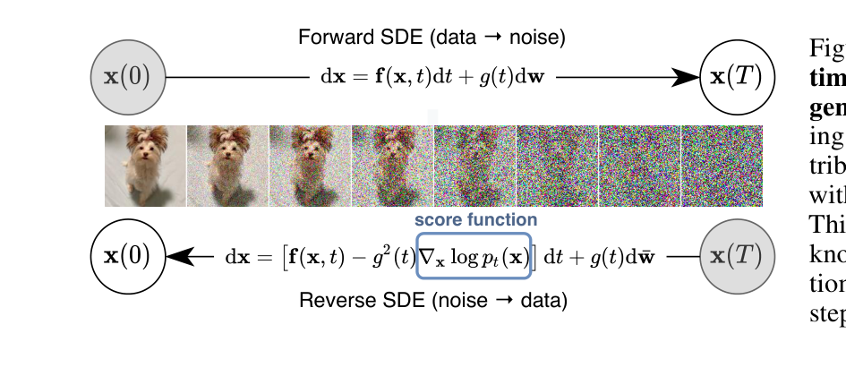
图源：Score-Based Generative Modeling through Stochastic Differential Equations，Figure 1。原论文图意：前向 SDE 把数据逐渐扩散为噪声；只要知道中间分布的 score，反向 SDE 就能从噪声生成数据。

这张图怎么读

输入输出：输入是数据分布与固定的加噪 SDE，输出是一个可从 prior 噪声反向生成数据的 SDE。
效率机制：它不是直接省掉训练，而是把采样问题变成可选择数值求解器的问题。
对主线意义：后续少步 solver、ODE sampler、distillation 和 flow matching 都是在这个连续时间视角里讨论“路径怎么走得更快”。
不能证明什么：一条漂亮的反向 SDE 不等于具体模型已低延迟、低 NFE 或可部署。

总体框架

论文 Figure 2 把三件事放在同一张图里：

前向 SDE：从 data 到 prior；
反向 SDE：从 prior 到 data；
probability flow ODE：一条确定性路径，和 SDE 有相同的边缘分布。

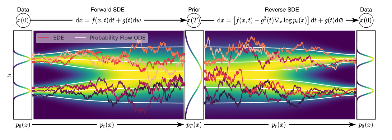
图源：Score-Based Generative Modeling through SDEs，Figure 2。原论文图意：数据可通过前向 SDE 映射到噪声 prior；反向 SDE 与 probability flow ODE 都可用 score $\nabla_x \log p_t(x)$ 构造。

这张图里最容易忽略的是白色曲线：它代表 probability flow ODE。反向 SDE 是随机的，每次采样路径会被噪声扰动；probability flow ODE 是确定性的，但在每个时间点拥有同样的边缘分布 $p_t(x)$ 。因此它能做三件 SDE 路径不方便做的事：

Capability	Why Probability Flow ODE Helps
Exact likelihood	Can use instantaneous change of variables as in neural ODEs
Latent encoding	A data point can be deterministically integrated to $x(T)$
Adaptive sampling	Black-box ODE solvers can trade tolerance for NFE

对应 ODE 为：

$dx = \left[ f(x,t)-\frac{1}{2}g(t)^2\nabla_x\log p_t(x) \right]dt.$

和反向 SDE 相比，区别是 score 项前面的系数从 $1$ 变成 $\frac{1}{2}$ ，并且没有随机 Wiener 项。

训练目标

训练时并不需要直接知道 $p_t(x)$ 的归一化密度。论文使用 denoising score matching 的连续时间形式：

$\theta^* = \arg\min_\theta \mathbb E_t \left\{ \lambda(t) \mathbb E_{x(0)} \mathbb E_{x(t)\mid x(0)} \left[ \left\lVert s_\theta(x(t),t) - \nabla_{x(t)} \log p_{0t}(x(t)\mid x(0)) \right\rVert_2^2 \right] \right\}.$

这条式子的读法是：

Term	Meaning
$t\sim U[0,T]$	随机抽一个连续噪声时刻
$x(0)\sim p_0$	从真实数据取 clean sample
$x(t)\sim p_{0t}(x(t)\mid x(0))$	按前向 SDE 加噪到时刻 $t$
$\nabla_{x(t)}\log p_{0t}(x(t)\mid x(0))$	对这次 perturbation kernel 的真实 denoising score
$s_\theta(x(t),t)$	神经网络预测的 time-dependent score
$\lambda(t)$	不同噪声时刻的 loss weight

关键点：如果前向 SDE 的 transition kernel $p_{0t}(x(t)\mid x(0))$ 是 Gaussian，训练就很方便，因为真实 denoising score 有闭式解。论文重点使用的 VE、VP、sub-VP SDE 都满足这个性质。

三类 SDE

论文把 SMLD 和 DDPM 分别解释成两类 SDE 的离散化，并引入 sub-VP SDE 改善 likelihood。

SDE	Forward Process	Discrete Ancestor	Main Behavior	Practical Role
VE SDE	$dx=\sqrt{\frac{d[\sigma^2(t)]}{dt}}dw$	SMLD / NCSN	variance exploding; signal mean roughly fixed while noise grows	strong sample quality with NCSN++
VP SDE	$dx=-\frac{1}{2}\beta(t)xdt+\sqrt{\beta(t)}dw$	DDPM	variance preserving when data variance is normalized	connects directly to DDPM-style training and sampling
sub-VP SDE	$dx=-\frac{1}{2}\beta(t)xdt+\sqrt{\beta(t)(1-e^{-2\int_0^t\beta(s)ds})}dw$	proposed in this paper	lower variance than VP at intermediate times	stronger likelihood in reported CIFAR-10 setting

这个表对工程判断很有用：**SDE 不是纯理论装饰，它会改变采样质量、likelihood 和最佳架构选择。**论文里 VE SDE 更偏向生成质量，sub-VP SDE 更偏向 likelihood。

采样：Predictor-Corrector

有了 score 网络后，可以用任意数值 SDE solver 近似反向 SDE。论文进一步提出 Predictor-Corrector sampler：

predictor:
  用数值 SDE solver 从 t_i 走到 t_{i-1}

corrector:
  在同一个噪声时刻，用 Langevin MCMC / HMC 之类 score-based MCMC 修正 marginal distribution

直觉上，predictor 负责沿时间方向往回走，corrector 负责在当前噪声层上“横向校正”样本，让样本更贴近 $p_t(x)$ 。这解释了为什么 PC sampler 在同等或相近 NFE 下常常比只加 predictor 更稳。

论文 Table 1 比较了 CIFAR-10 上不同 reverse-time SDE solvers。下面按原英文列名重绘。

Predictor	VE P1000	VE P2000	VE C2000	VE PC1000	VP P1000	VP P2000	VP C2000	VP PC1000
ancestral sampling	4.98 ± .06	4.88 ± .06	-	3.62 ± .03	3.24 ± .02	3.24 ± .02	-	3.21 ± .02
reverse diffusion	4.79 ± .07	4.74 ± .08	20.43 ± .07	3.60 ± .02	3.21 ± .02	3.19 ± .02	19.06 ± .06	3.18 ± .01
probability flow	15.41 ± .15	10.54 ± .08	-	3.51 ± .04	3.59 ± .04	3.23 ± .03	-	3.06 ± .03

表源：Score-Based Generative Modeling through SDEs，Table 1。原论文表意：P1000 / P2000 是 predictor-only，C2000 是 corrector-only，PC1000 是 1000 predictor steps + 1000 corrector steps；指标是 CIFAR-10 FID，越低越好。

这张表不应该读成“某个 sampler 永远最好”。更稳的读法是：

corrector-only 很贵而且效果差；
PC 通常比只增加 predictor steps 更值得；
probability flow 单独作为固定步 predictor 未必最好，但和 corrector 搭配时很强；
sampler 的好坏依赖 SDE、模型、步数和 SNR 超参。

Probability Flow ODE

probability flow ODE 的价值有两层。第一，它把扩散模型和 neural ODE、normalizing flow 的工具连接起来，可以算 exact likelihood。第二，它给采样提供了 adaptive NFE 的空间。

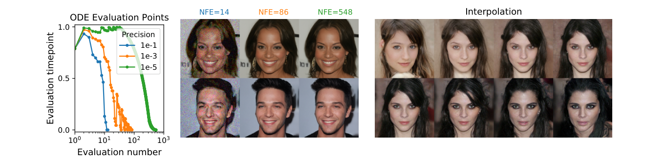
图源：Score-Based Generative Modeling through SDEs，Figure 3。原论文图意：ODE solver 的 evaluation points 可随数值精度变化；较少 NFE 仍可保持视觉质量；确定性 latent-to-image 映射支持 interpolation。

这张图怎么读

左图说明 ODE solver 会自动把函数评估集中到需要更高精度的时间段；中图显示从 NFE 548 降到 86 视觉质量仍接近，NFE 14 则明显退化；右图展示 deterministic encoding/decoding 支持 latent interpolation。它支撑的是“ODE 视角带来效率和表示能力”，不是“14 NFE 已经足够所有任务”。

论文 Table 2 报告了 probability flow ODE 用于 likelihood 和 ODE sampling 的结果。下面保留原英文表头。

Model	NLL Test ↓	FID ↓
RealNVP (Dinh et al., 2016)	3.49	-
iResNet (Behrmann et al., 2019)	3.45	-
Glow (Kingma & Dhariwal, 2018)	3.35	-
MintNet (Song et al., 2019b)	3.32	-
Residual Flow (Chen et al., 2019)	3.28	46.37
FFJORD (Grathwohl et al., 2018)	3.40	-
Flow++ (Ho et al., 2019)	3.29	-
DDPM (L) (Ho et al., 2020)	≤ 3.70*	13.51
DDPM (Lsimple) (Ho et al., 2020)	≤ 3.75*	3.17
DDPM	3.28	3.37
DDPM cont. (VP)	3.21	3.69
DDPM cont. (sub-VP)	3.05	3.56
DDPM++ cont. (VP)	3.16	3.93
DDPM++ cont. (sub-VP)	3.02	3.16
DDPM++ cont. (deep, VP)	3.13	3.08
DDPM++ cont. (deep, sub-VP)	2.99	2.92

表源：Score-Based Generative Modeling through SDEs，Table 2。* 表示 DDPM 原文的 ELBO 值是在 discrete data 上报告，论文正文特别说明这一点。

这里要注意一个很实际的 tradeoff：最佳 likelihood 不是最佳 FID。DDPM++ cont. (deep, sub-VP) 的 likelihood 最好，但 CIFAR-10 sample quality 最强的是 NCSN++ cont. (deep, VE)。

架构与训练细节

这篇论文的训练细节很值得单独看，因为它的结果不是“只改理论就赢了”，而是理论、采样器、架构和训练 recipe 叠加出来的。

基础训练设置

论文 Appendix H.1 给了架构探索设置：

Item	Setting
Architecture exploration iterations	`1.3M` unless otherwise noted
Checkpoint interval	every `50k` iterations
VE datasets	CIFAR-10 `32×32`, CelebA `64×64`
VP architecture search	CIFAR-10 only, to save compute
FID evaluation	`50k` samples, `tensorflow_gan`
Default architecture-search batch size	`128`
Sampler for architecture search	PC sampler with `1000` time steps
Predictor	reverse diffusion
VE corrector	one Langevin corrector step per predictor update, SNR `0.16`
VP corrector	usually omitted in architecture search to save doubled compute
Optimizer family	follows Ho et al. (2020): learning rate, gradient clipping, warm-up schedule

官方代码里的 CIFAR-10 default config 进一步给出常用训练超参：

Config Field	Value
`training.batch_size`	`128`
`training.n_iters`	`1300001` by default; deep continuous VE uses `950001`
`training.n_jitted_steps`	`5`
`model.sigma_min` / `model.sigma_max`	`0.01` / `50` for CIFAR-10 VE
`model.num_scales`	`1000`
`optim.optimizer`	`Adam`
`optim.lr`	`2e-4`
`optim.beta1` / `optim.eps`	`0.9` / `1e-8`
`optim.warmup`	`5000`
`optim.grad_clip`	`1.0`

这些细节对复现很重要。比如同样叫 NCSN++ cont.，如果训练步数、EMA、SNR、predictor/corrector 选择或 continuous embedding 不一致，FID 差距可能非常明显。

NCSN++ / DDPM++ 的设计

论文在 DDPM U-Net 体系上测试了几类架构组件：

FIR anti-aliasing upsampling/downsampling；
skip connection 乘 $1/\sqrt{2}$ 做 rescale；
把 DDPM residual block 换成 BigGAN residual block；
每个 resolution 的 residual blocks 从 2 增到 4；
测试 input / output 的 progressive architecture。

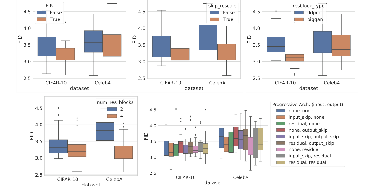
图源：Score-Based Generative Modeling through SDEs，Figure 10。原论文图意：在 VE perturbations 下，不同 architecture components 对 CIFAR-10 和 CelebA FID 的影响。

这张训练 ablation 图怎么读

图里多数橙色配置比蓝色配置 FID 更低，说明这些组件不是装饰项：FIR、skip rescale、BigGAN block、更多 residual blocks 都能影响 score model 的质量。这里的结论更像训练配方筛选，而不是新的理论定理。

最终命名可以这样记：

Model	Main Architecture Choice	SDE
NCSN++	FIR + skip rescale + BigGAN residual block + 4 res blocks/resolution + residual progressive input	VE
DDPM++	Similar search space, but best VP config drops FIR and progressive growing	VP / sub-VP
NCSN++ cont.	NCSN++ with continuous objective and random Fourier time embedding	VE
NCSN++ cont. (deep)	doubles residual blocks per resolution, trained `0.95M` iterations	VE
DDPM++ cont. (deep)	continuous DDPM++ with doubled depth	VP / sub-VP

连续时间条件的实现细节也很关键。论文把离散 timestep positional embedding 改成 random Fourier feature embeddings，scale 固定为 16。官方 deep continuous VE config 中，NCSN++ cont. (deep) 使用 nf=128、ch_mult=(1,2,2,2)、num_res_blocks=8、attn_resolutions=(16,)、dropout=0.1、scale_by_sigma=True 和 ema_rate=0.999。

EMA、过拟合和 checkpoint 选择

论文强调 EMA 对性能影响明显：

Setting	EMA
VE perturbations	`0.999` works better
VP perturbations	`0.9999` works better
1024×1024 CelebA-HQ	`0.9999`

还有一个容易漏掉的评测细节：Table 3 的 FID / IS 用的是训练过程中 FID 最低的 checkpoint；Table 2 的 likelihood 和 ODE FID 用的是最后 checkpoint。因此不能把两个表里的数字当成同一个 checkpoint 的全面画像。

CIFAR-10 sample quality

论文 Table 3 展示了最重要的 sample quality 结果。下面保留原英文表头。

Model	FID ↓	IS ↑
BigGAN (Brock et al., 2018), Conditional	14.73	9.22
StyleGAN2-ADA (Karras et al., 2020a), Conditional	2.42	10.14
StyleGAN2-ADA (Karras et al., 2020a), Unconditional	2.92	9.83
NCSN (Song & Ermon, 2019)	25.32	8.87 ± .12
NCSNv2 (Song & Ermon, 2020)	10.87	8.40 ± .07
DDPM (Ho et al., 2020)	3.17	9.46 ± .11
DDPM++	2.78	9.64
DDPM++ cont. (VP)	2.55	9.58
DDPM++ cont. (sub-VP)	2.61	9.56
DDPM++ cont. (deep, VP)	2.41	9.68
DDPM++ cont. (deep, sub-VP)	2.41	9.57
NCSN++	2.45	9.73
NCSN++ cont. (VE)	2.38	9.83
NCSN++ cont. (deep, VE)	2.20	9.89

表源：Score-Based Generative Modeling through SDEs，Table 3。原论文表意：NCSN++ cont. (deep, VE) 在 CIFAR-10 unconditional generation 上取得 FID 2.20 和 IS 9.89。

高分辨率训练

论文还把 NCSN++ 推到 $1024\times1024$ CelebA-HQ。这里训练设置和 CIFAR-10 明显不同：

Item	1024×1024 CelebA-HQ Setting
Model	modified NCSN++ with continuous objective
SDE	VE SDE
Batch size	`8`
EMA	`0.9999`
Training length	around `2.4M` iterations
Sampler	PC sampler with `2000` discretization steps
Predictor	reverse diffusion
Corrector	one Langevin step per predictor update
SNR	`0.15`
Fourier feature scale	`16`
Progressive architecture	`input skip` for input, `output skip` for output

{ width=“620” .atlas-figure-tall }

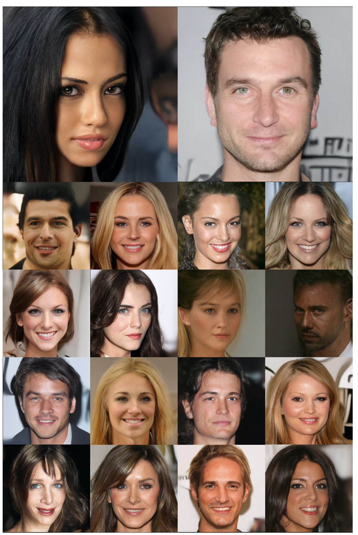
图源：Score-Based Generative Modeling through SDEs，Figure 12。原论文图意：使用 VE SDE 训练的 modified NCSN++ 在 $1024\times1024$ CelebA-HQ 上生成的样例。

论文自己也承认这些高分辨率样本并不完美，比如人脸对称性仍有可见瑕疵。这个表述很重要：它证明了 score-based model 可以上到 1024 分辨率，但还不是说它在视觉质量、速度和可控性上全面超过 GAN。

Controllable Generation

这篇论文还展示了一个很强的接口：如果你知道条件 $y$ 和当前 noisy state $x(t)$ 的关系，就可以把反向 SDE 改成条件反向 SDE：

$dx = \left\{ f(x,t) -g(t)^2 \left[ \nabla_x \log p_t(x) +\nabla_x\log p_t(y\mid x) \right] \right\}dt +g(t)d\bar w.$

这和后来的 guidance 思想非常接近：基础 score $\nabla_x\log p_t(x)$ 负责生成自然图像，条件梯度 $\nabla_x\log p_t(y\mid x)$ 负责把样本推向满足条件的区域。

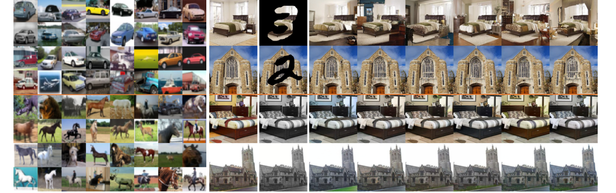
图源：Score-Based Generative Modeling through SDEs，Figure 4。原论文图意：左侧是 CIFAR-10 class-conditional samples；右侧是 LSUN 上的 inpainting 和 colorization。

三类应用分别是：

Task	Conditioning Signal	Extra Training?	Mechanism
Class-conditional generation	class label $y$	train time-dependent classifier	add $\nabla_x\log p_t(y\mid x)$ to reverse SDE
Inpainting	known pixels $\Omega(y)$	no new score model	constrain / resample known dimensions during reverse process
Colorization	grayscale observation	no new score model	transform channels to decouple known and unknown dimensions, then impute

这部分对后续 diffusion guidance 很有启发：扩散模型的条件控制不一定要在训练阶段全部做完，很多条件可以在反向过程里以梯度或 projection 方式注入。

训练实现清单

如果要按这篇论文复现或迁移到新任务，建议把训练拆成下面这张 checklist。

Stage	Decision
Choose SDE	VE for sample quality baseline; VP / sub-VP when likelihood or DDPM compatibility matters
Choose objective	continuous denoising score matching for modern SDE-style training
Time embedding	random Fourier features for continuous $t$ , scale `16` in reported configs
Network	U-Net family with residual blocks, attention at selected resolutions, EMA, dropout
Weighting	$\lambda(t)$ should balance score magnitude across noise levels
Sampler during eval	PC sampler for best quality; probability flow ODE for likelihood / latent / adaptive NFE
Corrector tuning	SNR is a real hyperparameter; official README notes typical `0.05-0.2`
Checkpointing	monitor FID across checkpoints, because the best sample checkpoint may not be the last
Report separately	sample FID / IS, ODE FID, NLL bits/dim, NFE, sampler steps

这张清单的核心是：SDE、训练目标、架构和 sampler 不能分开调。只换 sampler 不改 SDE，或只换 SDE 不调 EMA/SNR/embedding，都可能得到完全不同的结论。

和后续论文的关系

Later Direction	What It Inherits from Score SDE
DPM-Solver / DPM-Solver++	diffusion sampling as solving ODE/SDE with better numerical integration
Consistency models / distillation	learn a faster mapping along a continuous-time generative path
DMD / DMD2 / Phased DMD	use score models and diffusion perturbations as distribution-matching signals
CausVid / video diffusion acceleration	treat video diffusion sampling as a path that can be causalized, cached, or distilled
Flow matching / rectified flow	asks whether the generative path can be made straighter or easier than diffusion paths

可以把这篇论文看成扩散模型的“坐标系论文”。它未必是今天最快的生成方法，但它让后面很多方法都能在同一个坐标里比较：路径、score、noise schedule、ODE/SDE solver、NFE、likelihood、distillation。

局限与不可外推结论

论文提升了 score-based model 的质量和表达能力，但采样仍慢于 GAN，这是作者在结论里明确承认的限制。
PC sampler 的效果依赖 predictor、corrector、SNR、步数和 SDE；不能只引用 Table 1 的最优数字。
probability flow ODE 能算 likelihood，但最佳 likelihood 模型不等于最佳 FID 模型。
高分辨率 CelebA-HQ 结果证明了可扩展性，但样本仍有人脸对称性等瑕疵，不能外推出任意高分辨率域都稳定。
class-conditional generation 需要额外训练 time-dependent classifier；inpainting/colorization 虽可用 unconditional score model，但仍依赖任务结构和 projection / approximation 设计。
这篇论文主要是图像生成和逆问题证据，不能直接推出视频、3D、机器人世界模型中的时序一致性、动作因果或闭环收益。

读完接哪里

下一步

想补数学主线：读 Score Matching 到 SDE。
想看训练细节：读扩散训练与表示和扩散训练配方与排障。
想看采样加速：接 DPM-Solver++。
想看少步蒸馏：接 DMD、DMD2 和 Phased DMD。

这一页最后回到三个验收点：方法上，主公式是 forward SDE 加噪、reverse-time SDE 用 score 去噪，probability-flow ODE 则给出确定性采样和 likelihood 路径。实验上，图像生成、补全、上色和可控生成共同证明 score 不是只服务一种任务。诊断上，predictor-corrector、SDE/ODE 路径和 architecture component 的对比，才是理解后续 solver 与蒸馏论文的入口。

本站判断

Score SDE 是扩散统一理论页：方法要抓 forward SDE、reverse-time SDE、probability-flow ODE 和 predictor-corrector 采样；实验说明同一 score 框架能覆盖图像生成、补全和可控任务。后续论文多是在这套公式上换参数化、求解器或蒸馏目标。