
matlab-note-4
matlab-note-4
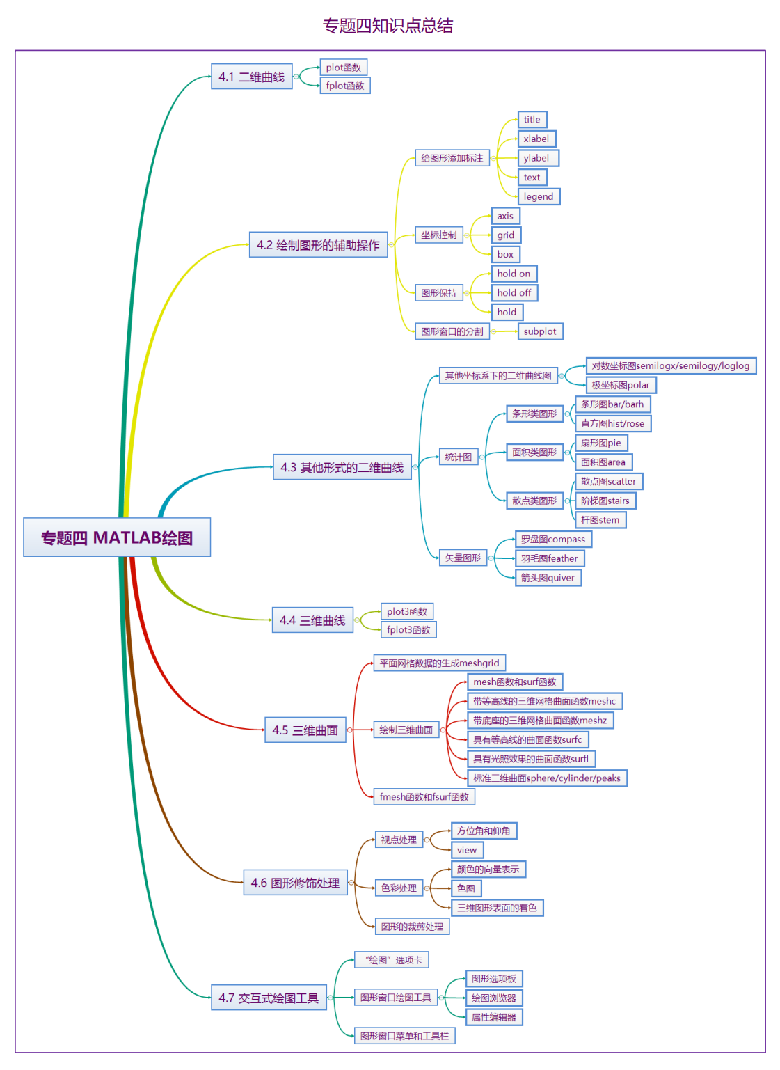
MATLAB绘图
二维曲线
plot函数
plot函数的基本用法:
其中,x和y分别用于存储x坐标和y坐标数据
1 | x = [2.5, 3.5, 4, 5]; |
最简单的plot函数调用格式
绘制函数元素下标为x轴,对应的值为y轴坐标。
1 | x = [1.5, 2, 1, 1.5]; |
当plot函数的参数x为复数向量时,则分别以该向量元素的实部和虚部为横、纵坐标绘制出一条曲线。
1 | x = [2.5, 3.5, 4, 5]; |
当x是向量,y是矩阵时
- 如果矩阵y的列数等于x的长度,则以向量x为横坐标,以y的每个行向量为纵坐标绘制曲线,曲线的条数等于y的行数。
- 如果矩阵y的行数等于x的长度,则以向量x为横坐标,以y的每个列向量为纵坐标绘制曲线,曲线的条数等于y的列数。
绘制sinx,sin(2x),sin(x/2)的函数曲线
1 | x = linspace(0, 2 * pi, 100); |
含选项的plot函数:plot(x,y,选项)
线型:"-":实线,":":虚线,"-.":点画线,"–":双画线。
颜色:“r”:红色,“g”:绿色,“b”:蓝色,“w”:白色,“k”:黑色……
数据点标记:"*":星号,“o”:圆圈,“s”:方块,“p”:五角星,"^":朝上三角符号……
1 | x = (0:pi / 50:2 * pi)'; |
fplot函数
fplot函数相比于plot函数的优势在于可以灵活的设置采样间隔以正确的反映图像的趋势。
fplot函数的基本用法
其中,f代表一个函数,通常采用函数句柄的形式。lims为x轴的取值范围,用二元向量[xmin,xmax]描述,默认值为[-5,5]。选项定义与plot函数相同。
1 | fplot(@(x)sin(1 ./ x), [0, 0.2], 'b') |
双输入函数参数的用法
其中,funx、funy代表函数,通常采用函数句柄的形式。tlims为参数函数funx和funy的自变量的取值范围,用二元向量[tmin,tmax]描述。
1 | fplot(@(t)t .* sin(t), @(t)t .* cos(t), [0, 10 * pi], 'r') |
绘制图形的辅助操作
图形标注
title(图形标题,属性名,属性值)【在图形标题中可以使用LaTex格式控制符】
color属性:用于设置图形标题文本的颜色。
fontsize属性:用于设置标题文字的字号。
xlabel(x轴说明)
ylabel(y轴说明)
text(x,y,图形说明)
legend(图例1,图例2,……)
“\bf”:加粗, “\it”:斜体, “\rm”:正体。
1 | x = -2 * pi:0.05:2 * pi; |
1 | x = linspace(0, 2 * pi, 100); |
坐标控制
axis函数:axis([xmin,xmax,ymin,ymax,zmin,zmax])
axis equal:纵、横坐标轴采用等长刻度。
axis square:产生正方形坐标系(默认为矩阵)
axis auto:使用默认设置
axis off:取消坐标轴
axis on:显示坐标轴
1 | x = [0, 1, 1, 0, 0]; |
给坐标系加网格:grid on,grid off,grid;
给坐标系加边框:box on,box off,box;
图形保持
hold on,hold off,hold;
1 | t = linspace(0, 2 * pi, 100); |
图形窗口的分割
subplot函数: ,其中,m和n指定将图形窗口分成个绘图区,p指定当前活动区。
1 | subplot(2, 2, 1); |
其他形式的二维图形
其他坐标系下的二维曲线图
对数坐标图
semilogx(x1,y1,option1,x2,y2,option2……)
semilogy(x1,y1,option1,x2,y2,option2……)
loglog(x1,y1,option1,x2,y2,option2……)其中,semilogx函数x轴为常用对数刻度,y轴为线性刻度;semilogy函数x轴为线性刻度,y轴为常用对数刻度;loglog函数x轴和y轴均采用常用对数刻度。
2
3
4
5
6
7
8
9
10
11
12
13
14
15
16
17
y = 1 ./ x;
subplot(2, 2, 1);
plot(x, y)
title('plot(x,y)');
subplot(2, 2, 2);
semilogx(x, y)
title('semilogx(x,y)');
grid on
subplot(2, 2, 3);
semilogy(x, y)
title('semilogy(x,y)');
grid on
subplot(2, 2, 4);
loglog(x, y)
title('loglog(x,y)');
grid on极坐标图
polar(theta,rho,option)其中,theta为极角,rho为极径,选项的内容与plot函数相同。
2
3
4
5
6
7
8
r = 1 - sin(t);
subplot(1, 2, 1);
polar(t, r)
subplot(1, 2, 2);
t1 = t - pi / 2;
r1 = 1 - sin(t1);
polar(t, r1)
统计图
条形图
bar函数:bar(x,y,style) x为横坐标,y是数据,style为指定分组排列模式。(绘制条形图还可以使用barh函数)
- bar函数:绘制垂直条形图。
- barh函数:绘制水平条形图。
1 | x = [2015, 2016, 2017]; |
直方图
hist函数(直角坐标系下):hist(y,x):参数y是要统计的数据,x用于指定区间的划分方式。
1 | y = randn(500, 1); |
rose函数(极坐标系下):rose(theta,x):theta用于确定每一区间与原点的角度,选项x用于指定区间的划分方式。
1 | y = randn(500, 1); |
扇形图
pie函数:pie(x,explode) ,其中,参数x存储待统计数据,选项explode控制图块的显示模式。
1 | score = [5, 17, 23, 9, 4]; |
面积图
area函数(用法和plot函数相同)
散点图
scatter函数(用法和plot函数相同)
scatter(x, y, 选项, ‘filled’)
其中,x、y用于定位数据点,选项用于指定线型、颜色、数据点标记。如果数据点标记是封闭图形,可以用选项‘filled’指定填充数据点标记。该选项省略时,数据点是空心的。
1 | t = 0:pi / 50:2 * pi; |
阶梯图
stairs函数(用法和plot函数相同)
杆图
stem函数(用法和plot函数相同)
矢量图形
罗盘图
compass函数
羽毛图
feather函数
箭头图
quiver函数: quiver(x,y,u,v) 其中,(x,y)指定矢量起点,(u,v)指定矢量终点。x、y、u、v是同样大小的向量或同型矩阵,若省略x、y,则在x-y平面上均匀取若干个点作为起点。
1 | A = [4, 5]; B = [-10, 0]; C = A + B; |
三维曲线
可以利用plot3函数和fplot3函数进行绘图,用法可以参考(plot和fplot函数)
1 | x = [0.2, 1.8, 2.5]; |
1 | xt = @(t) exp(-t / 10) .* sin(5 * t); |
三维曲面
平面网格数据的生成
1.利用矩阵运算生成
1 | x = 2:6; |
2.利用meshgrid函数生成
其中,参数x,y为向量,存储网格点坐标的X,Y为矩阵。
1 | x = 2:6; |
绘制三维曲线的函数
mesh(x,y,z,c):三维网格图绘制
surf(x,y,z,c):三维曲面图绘制
其中x,y,z是网格坐标矩阵,z是网格点上的高度矩阵,c用于指定不同高度下的曲面颜色。
当x、y省略时,z矩阵的第2维下标当做x轴坐标,z矩阵的第1维下标当做y轴坐标。
1 | t = -2:0.2:2; |
meshc函数:带等高线的三维网格曲面函数。
meshz函数:带底座的三维网格曲面函数。
surfc函数:带等高线的曲面函数。
surfl函数:带光照效果的曲面函数。
1 | [x, y] = meshgrid(0:0.1:2, 1:0.1:3); |
标准三维曲面
sphere函数:三维球面
产生3个(n+1)阶的方阵,采用这3个矩阵可以绘制出圆心位于原点、半径为1的单位球体。
cylinder函数:三维柱面
其中,参数R是一个向量,存放柱面各个等间隔高度上的半径,n表示在圆柱圆周上有n个间隔点,默认有20个间隔点。
1 | subplot(1, 3, 1); |
peaks函数:多峰函数
1 | p1 = peaks(10); |
fsurf函数和fmesh函数
用于绘制参数方程定义的曲面
其中,funx、funy、funz代表定义曲面x、y、z坐标的函数,通常采用函数句柄的形式。uvlims为funx、funy和funz的自变量的取值范围,用4元向量[umin, umax, vmin, vmax]描述,默认为[-5, 5, -5, 5]。
1 | funx = @(u, v) u .* sin(v); |
图形修饰处理
视点处理
方位角:视点与原点连线在xy平面上的投影与y轴负方向形成的角度,正值表示逆时针,负值表示顺时针。
仰角:视点与原点连线与xy平面的夹角,正值表示视点在xy平面上方,负值表示视点在xy平面下方。
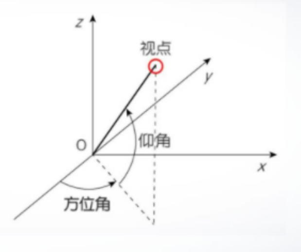
view函数的基本用法: 其中,az为方位角,el为仰角。系统默认的视点定义为方位角-37.5°,仰角30°。
1 | [x, y] = meshgrid(0:0.1:2, 1:0.1:3); |
色彩处理
1.颜色的向量表示(RGB表示)
向量元素在[0,1]范围内取值,3个元素依次表示红、绿、蓝3种颜色的相对亮度,称为RGB三元组。
2.色图(colormap)
colormap cmapname
1 | surf(peaks) |
这种类似于颜色自定义
1 | c = [0, 0.2, 0.4, 0.6, 0.8, 1]'; |
3.三维图片表面的着色
可以用shading函数来改变着色方式。
shading faceted:每个网格片用其高度对应的颜色进行着色,网格线是黑色。这是默认着色方式。
shading flat:每个网格片用同一个颜色进行着色,且网格线也用相应的颜色。
shading interp:网格片内采用颜色插值处理。
1 | [x, y, z] = cylinder(pi: -pi / 5:0, 10); |
裁剪处理
将图形中需要裁剪部分对应的函数数值设置为NaN,这样在绘制图形时,函数值为NaN的部分将不会显示出来,从而达到对图形进行裁剪的目的。
1 | t = linspace(0, 2 * pi, 100); |
通过y§ = NaN;裁剪
交互式绘图工具
"绘图"选项卡
“绘图”选项卡的工具条提供了绘制图形的基本命令。
- “所选内容”命令组:用于显示已选中用于绘图的变量;
- “绘图”命令组:提供了绘制各种图形的命令;
- “选项”命令组:用于设置绘图时是否新建图形窗口。
通过命令行输入plottools启动绘图工具
图形窗口绘图工具
图形窗口菜单和工具栏
图形绘制完成后,可以用“文件”菜单中的“生成代码”命令,将实施在图形上的这些操作命令输出成脚本。也可以用“保存”命令将图形窗口内容保存为fig文件。
- Title: matlab-note-4
- Author: Charles
- Created at : 2023-02-03 22:34:07
- Updated at : 2026-05-11 20:11:20
- Link: https://charles2530.github.io/2023/02/03/matlab-note-4/
- License: This work is licensed under CC BY-NC-SA 4.0.